Firms theory
Plan
- The Ownership and Management of Firms. How businesses are organized affects who makes decisions and the firm's objective, such as whether it tries to maximize profit.
- Production. A firm converts inputs into outputs using one of possibly many available technologies.
- Short-Run Production. In the short run, only some inputs can be varied, so the firm changes its output by adjusting its variable inputs.
- Long-Run Production. The firm has more flexibility in how it produces and how it changes its output level in the long run when all factors can be varied.
- Returns to Scale. How the ratio of output to input varies with the size of the firm is an important factor in determining the size of a firm.
- Productivity and Technical Change. The amount of output that can be produced with a given amount of inputs varies across firms and over time.
Production functions
Firm tries to maximize its profit, which equals to revenue minus cost.
A production function is the technology the firm has at its disposal to turn inputs into outputs. The inputs that it's going to take in are going to be capital K and labor L.
\(q = F(L,K)\).
Key distinction from Utility function.
- Inputs that are fixed.
-
Inputs that are variable.
- Short-run:
-
- Capital is fixed
-
- Labor is variable
- Long-run:
-
- Everything is variable
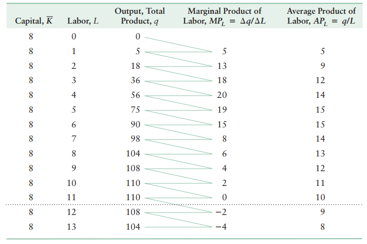
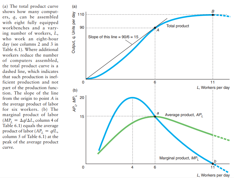
Marginal product of labor
The marginal product of labor is going to be the change in quantity produced for a given change in labor holding capital fix.
\(MP_L = \frac{\Delta q}{\Delta L} \vert_{\bar{K}}\).
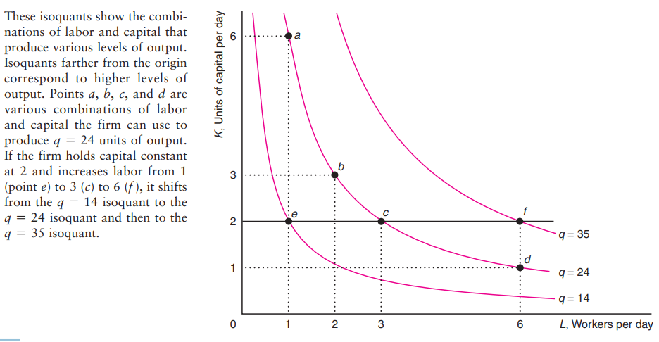
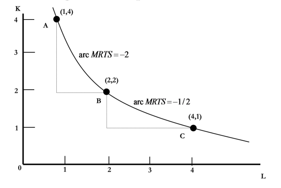
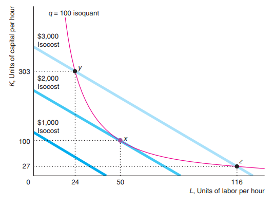
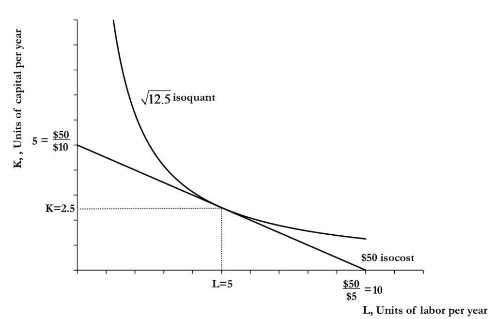
Isoquants
Isoquants are the firm's indifference curves, which is namely combinations of k and l which yield the same level of output.
MRTS
Returns to scale
- Constant returns to scale \(F(2L, 2K) = 2 F(L,K)\)
- Increasing returns to scale \(F(2L, 2K) > 2F(L,K)\). Example of when firm could exhibit IRS, is when firm start specializing in producing of products.
- Decreasing returns to scale \(F(2L, 2K) < 2 F(L,K)\). Example of when firm could exhibit DRS, is when firm gets bigger it is harder to manage employees hence productivity falls down.
Productivity
Costs
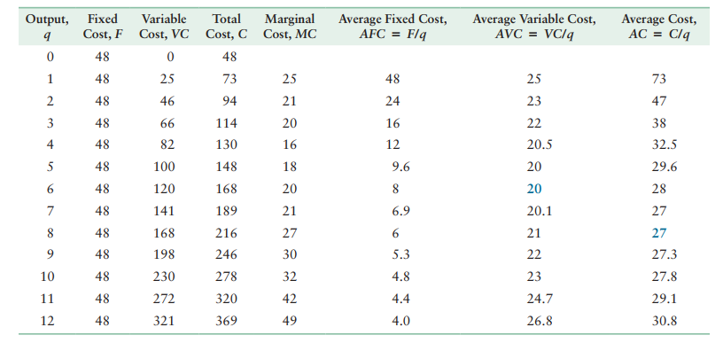
Fixed cost (FC) is a production expense that does not vary with output.
variable cost (VC) a production expense that changes with the quantity of output produced.
Cost (total cost, TC) the sum of a firm's variable cost and fixed cost: \(TC = FC + VC\).
Marginal cost (MC) the amount by which a firm's cost changes if the firm produces one more unit of output. \(MC = \frac{\Delta C}{\Delta q}\).
Average fixed cost (AFC) the fixed cost divided by the units of output produced: \(AFC = \frac{FC}{q}\).
Average variable cost (AVC) the variable cost divided by the units of output produced: \(AVC = \frac{VC}{q}\).
Average total cost (ATC) is the total cost divided by the units of output produced: \(ATC = \frac{TC}{q} = \frac{FC}{q} + \frac{VC}{q}\).
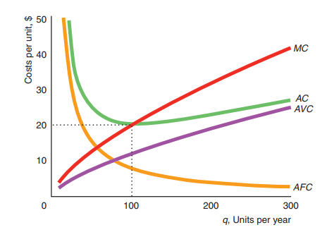
Short Run Cost Curves
Our short run production function \(q = F(L, \bar{K})\), where capital is fixed.
Cost of producing any given quantity \(TC = r*\bar{K} + w*L\), where r is renting price of the capital(per period cost of using a unit of capital) and w is the price of the labor.
\(MC = w * \frac{\Delta L}{\Delta q} \quad (1)\), since we defined \(MP_L = \frac{\Delta q}{\Delta L}\), we then can rewrite equation (1) as \(MC = w* \frac{1}{MP_L}\). We can see that marginal cost moves inversely with marginal product of labor. It happens because, the more producte one additional worker, the cheaper it will be to produce one additional item.
Example
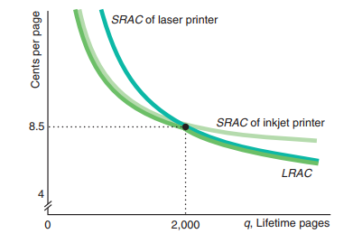
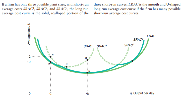
Long Run Cost Curves
In the long run capital and labor are variable inputs, so the firm should decide how much capital and labor it will need to produce given quantity of good. \
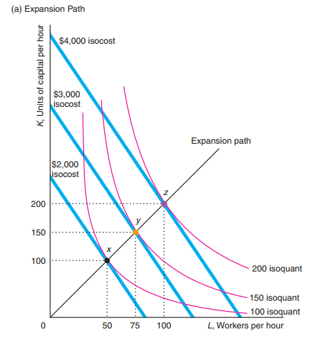
Isocost
Isocost curve is the combination of Labor and Capital that yield us the same cost.
\(C = r*K + w*L\).
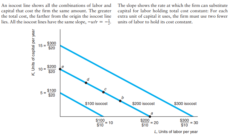
The point that minimizes your cost as a firm is the tangency between your isoquant and your isocost.
Cost minimization
The optimal bundle of labor and capital, given the quantity of goods, company going to produce is found by equation \(-\frac{MP_L}{MP_K} = -\frac{w}{r}\).
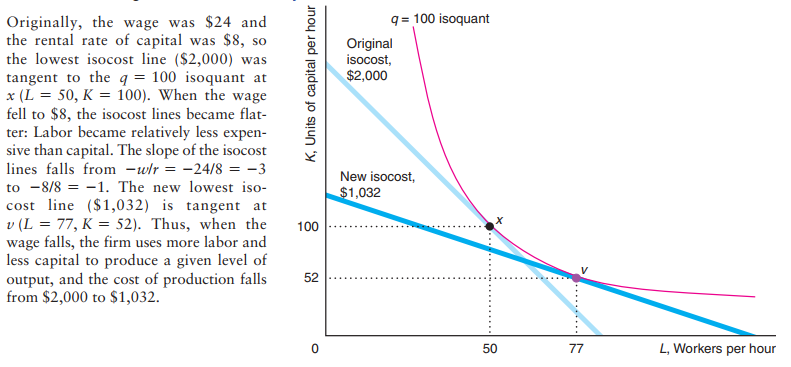
Change in factor price
Expansion path
Long run cost curve