Basics of R
Some materials are taken from the book "Hands-On-Programming With R" by Garrett Grolemund and online course on Coursera "Statistics with R"
Objects
R lets you save data by storing it inside an R object. What's an object? Just a name that you can use to call up stored data. For example, you can save data into an object like a or b. Wherever R encounters the object, it will replace it with the data saved inside, like so:
You can store numbers in objects, assume that you are paying 300$ for particular month in gas bills.
gas <- 300
gas
## [1] 300
Then suddenly fees are decreased.
gas <- 200
gas
## [1] 200
Assume that you are also paying for your groceries. Lets compute total expenditures in the month
groceries <- 2000
groceries
## [1] 2000
total = gas + groceries
total
## [1] 2200
You can also, store text data in objects. Text data should be in quotes.
name <- "Aibek"
You can see which object names you have already used with the function ls()
ls()
## [1] "gas" "groceries" "name" "total"
Naming conventions
You can name an object in R almost anything you want, but there are a few rules. First, a name cannot start with a number. Second, a name cannot use some special symbols, like ^, !, $, @, +, -, /, or *.
Sequence of numbers (Vectors)
Continious sequence of numbers
Objects can also store sequence of numbers. Assume that you have Alex, John, Sam. And their respecive ages are 18,19,20. You can store their ages in the object ages.
ages <- 18:20
ages
## [1] 18 19 20
Discrete sequence of numbers
Assume that Alex, John and Sam are respecitvely 17, 23, 25 years old. In the case when we have discrete set of numbers, we can still store this numbers in the object. To do that we need to use special operator c(). For example,
ages <- c(17, 23, 25)
ages
## [1] 17 23 25
One can remember usefull mnemonic to remember c() operator as first letter for the word column. Basically, when we use operator c() we created one column from spreadsheet by the name ages.
| ages |
|---|
| 17 |
| 23 |
| 25 |
R uses fancy name for columns, they are called vectors. So it is safely assume, that vectors are just columns of a spreadsheet.
In the same manner, we can create the column of names.
names <- c("Alex", "John", "Sam")
| names |
|---|
| Alex |
| John |
| Sam |
Dataframes
What is dataframe? Data is nothing more than just the spreadsheet. To create dataframe we can use command Data.Frame(). Inside of the round brackets we need to supply columns, from which our dataframe will consist. For example, let us create dataframe of names and ages of people.
ages <- c(17, 23, 25)
names <- c("Alex", "John", "Sam")
df <- Data.Frame(names, ages)
df
We will have output as,
| names | ages |
|---|---|
| Alex | 17 |
| John | 23 |
| Sam | 25 |
Working with missing values in R
names <- c("Alex", "John", "Michael", "Joe", "Wu")
wages <- c(30000, 25000, NA, 50000, 43000)
ages <- c(NA, 25, 23, 30, NA)
df <- data.frame(names, wages, ages)
head(df)
| names | wages | ages | |
|---|---|---|---|
| <fct> | <dbl> | <dbl> | |
| 1 | Alex | 30000 | NA |
| 2 | John | 25000 | 25 |
| 3 | Michael | NA | 23 |
| 4 | Joe | 50000 | 30 |
| 5 | Wu | 43000 | NA |
Number of missing values in each column
To check how much each column contains missing values, you can execute command, with supplied name of your dataframe. colSums(is.na(YOUR_DATAFRAME))
colSums(is.na(df))
names:0 wages:1 ages:2
We can see that there is 0 missing values in the column names. One missing value in the column wages and two missing values in the column ages.
Doing statistics with missing values.
You can use statistical function in your code, even if your column has missing values, however you need explicetly state to your function, that you have missing values.
mean(df$ages)
# NA
When we applied mean function to the column df\$ages we got _
mean(df$ages, na.rm = TRUE)
# 26
For loop
For loops command allows your code to run in loops. It makes your code more managable, short and clean.
Lets print the name of our fruits in a basket.
basket <- c('apple', 'banana', 'pineapple', 'grape', 'orange')
for(name in basket){
  print(name)
}
## [1] "apple"
## [1] "banana"
## [1] "pineapple"
## [1] "grape"
## [1] "orange"
Let's add word ‘is fruit' to each fruit in a loop.
for(name in basket){
  print( paste(name,'is fruit'))
}
## [1] "apple is fruit"
## [1] "banana is fruit"
## [1] "pineapple is fruit"
## [1] "grape is fruit"
## [1] "orange is fruit"
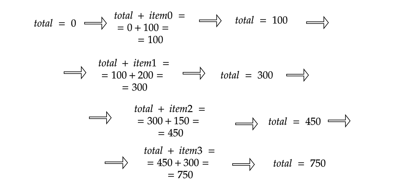
Let's compute total income in a loop.
income <- c(100, 200, 150, 300, 400, 300)
total <- 0
for(item in income){
  total <- total + item
}
print(total)
## [1] 1450
Picture below shows the way we increment income in a loop. First our initial income total=0, then we increment in a loop, using variable item that in each loop will take value from our income vector.
Functions
Function is just a word that encapsulates sets of instructions. When you execute your function, you will basically execute your sets of instructions. You can imagine functions as the cooking receipe. The process of cooking consists of:
- recipie, which in our case would be block of function encapsulated by a word.
- ingridients, which in our case would be
argumentsthat we supply to our function - finished cooked food that you need to serve, which in our case would be returned result from our function. The basic syntaxis of any function looks as follows,
cooking_apple_pie <- function(ingridient1, ingridient2){
	apple_pie <- cook_food_using_ingridients
	return apple_pie
}
As an example, let's create a function to calculate the length of the hypotenuse of a right-angled triangle.
hypotenuse <- function(a, b) {
    c <- sqrt(a^2+b^2)
    return(c)
    }
Let's compute length of hypotenuse of triangle with sides 3 and 4.
hypotenuse(3,4)
5