Econometric models

Probit and logit models

In the probit and logit models dependent variable is dummy variable (0 and 1). For example, whether you defaulted on your credit or not. Whether you are eligible for the program or not, etc etc.

Data source

For more details please refere to AER package documentation, page 140. link Cross-section data about resume, call-back and employer information for 4,870 fictitious resumes sent in response to employment advertisements in Chicago and Boston in 2001, in a randomized controlled experiment conducted by Bertrand and Mullainathan (2004). The resumes contained information concerning the ethnicity of the applicant. Because ethnicity is not typically included on a resume, resumes were differentiated on the basis of so-called "Caucasian sounding names" (such as Emily Walsh or Gregory Baker) and "African American sounding names" (such as Lakisha Washington or Jamal Jones). A large collection of fictitious resumes were created and the presupposed ethnicity (based on the sound of the name) was randomly assigned to each resume. These resumes were sent to prospective employers to see which resumes generated a phone call from the prospective employer.

Logit model

library(AER)
data(ResumeNames)
head(ResumeNames)
  

A data.frame: 6 × 27
	name	gender	ethnicity	quality	call	city	jobs	experience	honors	volunteer	...	minimum	equal	wanted	requirements	reqexp	reqcomm	reqeduc	reqcomp	reqorg	industry
	<fct>	<fct>	<fct>	<fct>	<fct>	<fct>	<int>	<int>	<fct>	<fct>	...	<fct>	<fct>	<fct>	<fct>	<fct>	<fct>	<fct>	<fct>	<fct>	<fct>
1	Allison	female	cauc	low	no	chicago	2	6	no	no	...	5	yes	supervisor	yes	yes	no	no	yes	no	manufacturing
2	Kristen	female	cauc	high	no	chicago	3	6	no	yes	...	5	yes	supervisor	yes	yes	no	no	yes	no	manufacturing
3	Lakisha	female	afam	low	no	chicago	1	6	no	no	...	5	yes	supervisor	yes	yes	no	no	yes	no	manufacturing
4	Latonya	female	afam	high	no	chicago	4	6	no	yes	...	5	yes	supervisor	yes	yes	no	no	yes	no	manufacturing
5	Carrie	female	cauc	high	no	chicago	3	22	no	no	...	some	yes	secretary	yes	yes	no	no	yes	yes	health/education/social services
6	Jay	male	cauc	low	no	chicago	2	6	yes	no	...	none	yes	other	no	no	no	no	no	no	trade

# encoding "call" column categorical levels into numerical
ResumeNames$call <- ifelse(ResumeNames$call == "yes", 1, 0)
# making logit model
model_logit <- glm(call ~ethnicity + gender + quality, data = ResumeNames)
summary(model_logit)
  

Call:
Call:
glm(formula = call ~ ethnicity + gender + quality, family = binomial(link = "logit"),
    data = ResumeNames)

Deviance Residuals:
    Min       1Q   Median       3Q      Max
-0.4770  -0.4356  -0.3867  -0.3525   2.4207

Coefficients:
              Estimate Std. Error z value Pr(>|z|)
(Intercept)    -2.4350     0.1348 -18.058  < 2e-16 ***
ethnicityafam  -0.4399     0.1074  -4.096  4.2e-05 ***
genderfemale    0.1276     0.1289   0.990   0.3222
qualityhigh     0.1914     0.1059   1.806   0.0709 .
---
Signif. codes:  0 '***' 0.001 '**' 0.01 '*' 0.05 '.' 0.1 ' ' 1

(Dispersion parameter for binomial family taken to be 1)

    Null deviance: 2726.9  on 4869  degrees of freedom
Residual deviance: 2705.7  on 4866  degrees of freedom
AIC: 2713.7

Number of Fisher Scoring iterations: 5
  

From the regression table we can see coefficient for ethnicityafam is -0.4399, that means that if the applicant have african american sounding name then he is less likely to recieve call back.

Warning

We can not interpret magnitude from the regression table for logit model, only we can interpret the direction of the effect i.e. more likely or less likely get called back.

Probit model

Probit models are pretty much similiar to logit models(see above). Just in the glm() command we need to specify the family argument to be family = binomial(link="logit").

model_probit <- glm(call ~ ethnicity + gender + quality, family = binomial (link="probit"), data = ResumeNames)
summary(model_probit)
  

Call:
glm(formula = call ~ ethnicity + gender + quality, family = binomial(link = "probit"),
    data = ResumeNames)

Deviance Residuals:
    Min       1Q   Median       3Q      Max
-0.4757  -0.4363  -0.3871  -0.3525   2.4225

Coefficients:
              Estimate Std. Error z value Pr(>|z|)
(Intercept)   -1.39798    0.06642 -21.047  < 2e-16 ***
ethnicityafam -0.21685    0.05282  -4.105 4.04e-05 ***
genderfemale   0.06208    0.06336   0.980   0.3272
qualityhigh    0.09305    0.05252   1.772   0.0764 .
---
Signif. codes:  0 '***' 0.001 '**' 0.01 '*' 0.05 '.' 0.1 ' ' 1

(Dispersion parameter for binomial family taken to be 1)

    Null deviance: 2726.9  on 4869  degrees of freedom
Residual deviance: 2705.8  on 4866  degrees of freedom
AIC: 2713.8

Number of Fisher Scoring iterations: 5
  

From the regression table we can see coefficient for ethnicityafam is -0.21685 (which is little bit different compared to logit model) that means that if the applicant have african american sounding name then he is less likely to recieve call back.

Warning

We can not interpret magnitude from the regression table for probit model, only we can interpret the direction of the effect i.e. more likely or less likely get called back.

Average marginal effects

To have meaningful interpretation of effects we can calculate average marginal effects.

Logit model

marginal_logit <- mean(dlogis(predict(model_logit, type="link")))
marginal_logit * coef(model_logit)
  

(Intercept) -0.179439881066858    ethnicityafam -0.324139363996093  genderfemale  0.00940104037935758  qualityhigh  0.0141013274125201
  

Interpretation of marginal effect for variable ethnicityafam is -0.324139363996093, which means if the person has african american sounding name, then he is 32% less likely to get call back from potential employer.

Probit model

marginal_probit <- mean(dnorm(predict(model_probit, type="link")))
marginal_probit * coef(model_probit)
  

(Intercept) -0.207308146098111 ethnicityafam -0.0321574328415445 genderfemale 0.00920546735038312 qualityhigh 0.0137988149880605
  

Interpretation of marginal effect for variable ethnicityafam is -0.0321574328415445, which means if the person has african american sounding name, then he is 32% less likely to get call back from potential employer.

Note

We can see that coefficient for logit and probit models could be quite different, but the average marginal effects are on contrary quite similliar.

Multinomial logit model

If the outcome variable is categorical variable without inherent oreder(regular categorical), such as car manufacturers. The we need to use multinomial logit model.

Data source

Data is on penguins and their characterstics. There is three type of penguins: Adelie, Gentoo and Chinstrap. Data were collected and made available by Dr. Kristen Gorman and the Palmer Station, Antarctica LTER, a member of the Long Term Ecological Research Network.

library(nnet)
df <- read.csv('https://raw.githubusercontent.com/mwaskom/seaborn-data/master/penguins.csv')
head(df)
  

multinom_logit <- multinom(species ~ bill_length_mm + flipper_length_mm + body_mass_g + sex, data = df)
summary(multinom_logit)
  

Call:
multinom(formula = species ~ bill_length_mm + flipper_length_mm +
    body_mass_g + sex, data = df)

Coefficients:
          (Intercept) bill_length_mm flipper_length_mm  body_mass_g sexFEMALE   sexMale
Chinstrap   -126.8121       3.884542        0.05522745 -0.013713867  1.140113   -9.134096
Gentoo      -190.0349       1.235787        0.59656936  0.005336206 -2.307075   -17.078332

Std. Errors:
          (Intercept) bill_length_mm flipper_length_mm body_mass_g  sexFEMALE   sexMALE
Chinstrap 0.031418912      1.0980540         0.1551344 0.006644753 0.06812109   0.03713893
Gentoo    0.007206881      0.9901455         0.2358709 0.006981574 0.08631697   0.03341686

Residual Deviance: 7.341373
AIC: 31.34137
  

These are the logit coefficients relative to the reference category. For example, under ‘body_mass_g', the 0.006644753 suggests that for one unit increase in ‘body_mass_g' weight, the logit coefficient for ‘Chinstrap' relative to ‘Adelie' will go up by that amount, 0.006644753. In other words, if your ‘body_mass_g' weight increases one unit, the chances of the penguin to be identified as ‘Chinstrap' compared to the chances of being identified as ‘Adelie' are higher.

Note

Multinom() function does not provide p-values. Either you can compute them customly, or you can use package stargazer, that computes p-values for you.

library(stargazer)
stargazer(multinom_logit, type="text")
  

==============================================
                      Dependent variable:
                  ----------------------------
                    Chinstrap       Gentoo
                       (1)            (2)
----------------------------------------------
bill_length_mm       3.885***        1.236
                     (1.098)        (0.990)

flipper_length_mm     0.055         0.597**
                     (0.155)        (0.236)

body_mass_g          -0.014**        0.005
                     (0.007)        (0.007)

sexFEMALE            1.140***      -2.307***
                     (0.068)        (0.086)

sexMALE             -9.134***     -17.078***
                     (0.037)        (0.033)

Constant           -126.812***    -190.035***
                     (0.031)        (0.007)

----------------------------------------------
Akaike Inf. Crit.     31.341        31.341
==============================================
Note:              *p<0.1; **p<0.05; ***p<0.01
  

Relative risk ratios

Relative risk ratios allow an easier interpretation of the logit coefficients. They are the exponentiated value of the logit coefficients.

multinom_logit_coeff <- exp(coef(multinom_logit))
stargazer(multinom_logit, type="text", coef=list(multinom_logit_coeff))
  

==============================================
                      Dependent variable:
                  ----------------------------
                    Chinstrap       Gentoo
                       (1)            (2)
----------------------------------------------
bill_length_mm        48.645         3.441
                     (1.098)        (0.990)

flipper_length_mm    1.057***      1.816***
                     (0.155)        (0.236)

body_mass_g          0.986***      1.005***
                     (0.007)        (0.007)

sexFEMALE            3.127***      0.100***
                     (0.068)        (0.086)

sexMALE             0.0001***     0.00000***
                     (0.037)        (0.033)

Constant              0.000          0.000
                     (0.031)        (0.007)

----------------------------------------------
Akaike Inf. Crit.     31.341        31.341
==============================================
Note:              *p<0.1; **p<0.05; ***p<0.01
  

If we look at the first row of the regression table, we can interpret it as following:
- keeping all other variables constant, if bill_length_mm varaible increases one unit(cm), you are 48.645 times more likely to be identified as Chinstrap penguin as compared to the Adelie penguins. The coefficient, however, is not significant.
- Keeping all other variables constant, if bill_length_mm varaible increases one unit(cm), you are 3.441 times more likely to be identified as Gentoo penguin as compared to the Adelie penguins. The coefficient, however, is not significant.

Mutlinomial probit model

Polynomial regression

In some cases, the true relationship between the outcome and a predictor variable might not be linear.

There are different solutions extending the linear regression model for capturing these nonlinear effects, including:

Polynomial regression. This is the simple approach to model non-linear relationships. It add polynomial terms or quadratic terms (square, cubes, etc) to a regression.
Spline regression. Fits a smooth curve with a series of polynomial segments. The values delimiting the spline segments are called Knots.
Generalized additive models (GAM). Fits spline models with automated selection of knots.

We'll use Boston data set. The median house value (mdev), in Boston Suburbs. Variable lstat (percentage of lower status of the population).

library(tidyverse)
data("Boston", package = "MASS")
head(Boston)
  

A data.frame: 6 × 14
	crim	zn	indus	chas	nox	rm	age	dis	rad	tax	ptratio	black	lstat	medv
	<dbl>	<dbl>	<dbl>	<int>	<dbl>	<dbl>	<dbl>	<dbl>	<int>	<dbl>	<dbl>	<dbl>	<dbl>	<dbl>
1	0.00632	18	2.31	0	0.538	6.575	65.2	4.0900	1	296	15.3	396.90	4.98	24.0
2	0.02731	0	7.07	0	0.469	6.421	78.9	4.9671	2	242	17.8	396.90	9.14	21.6
3	0.02729	0	7.07	0	0.469	7.185	61.1	4.9671	2	242	17.8	392.83	4.03	34.7
4	0.03237	0	2.18	0	0.458	6.998	45.8	6.0622	3	222	18.7	394.63	2.94	33.4
5	0.06905	0	2.18	0	0.458	7.147	54.2	6.0622	3	222	18.7	396.90	5.33	36.2
6	0.02985	0	2.18	0	0.458	6.430	58.7	6.0622	3	222	18.7	394.12	5.21	28.7

ggplot(Boston, aes(lstat, medv) ) +
  geom_point() +
  geom_smooth(method='lm')
  

png

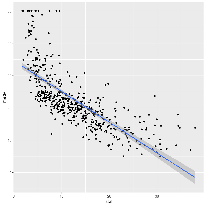
model <- lm(medv ~ lstat, data = Boston)
summary(model)
  

Call:
lm(formula = medv ~ lstat, data = Boston)

Residuals:
    Min      1Q  Median      3Q     Max
-15.168  -3.990  -1.318   2.034  24.500

Coefficients:
            Estimate Std. Error t value Pr(>|t|)
(Intercept) 34.55384    0.56263   61.41   <2e-16 ***
lstat       -0.95005    0.03873  -24.53   <2e-16 ***
---
Signif. codes:  0 '***' 0.001 '**' 0.01 '*' 0.05 '.' 0.1 ' ' 1

Residual standard error: 6.216 on 504 degrees of freedom
Multiple R-squared:  0.5441,	Adjusted R-squared:  0.5432
F-statistic: 601.6 on 1 and 504 DF,  p-value: < 2.2e-16
  

The polynomial regression adds polynomial or quadratic terms to the regression equation as follow:

\[medv = b0 + b1*lstat + b2*lstat^2\]

model_pol <- lm(medv ~ lstat + I(lstat^2), data = Boston)
summary(model_pol)
  

Call:
lm(formula = medv ~ lstat + I(lstat^2), data = Boston)

Residuals:
     Min       1Q   Median       3Q      Max
-15.2834  -3.8313  -0.5295   2.3095  25.4148

Coefficients:
             Estimate Std. Error t value Pr(>|t|)
(Intercept) 42.862007   0.872084   49.15   <2e-16 ***
lstat       -2.332821   0.123803  -18.84   <2e-16 ***
I(lstat^2)   0.043547   0.003745   11.63   <2e-16 ***
---
Signif. codes:  0 ‘***' 0.001 ‘**' 0.01 ‘*' 0.05 ‘.' 0.1 ‘ ' 1

Residual standard error: 5.524 on 503 degrees of freedom
Multiple R-squared:  0.6407,	Adjusted R-squared:  0.6393
F-statistic: 448.5 on 2 and 503 DF,  p-value: < 2.2e-16
  

model_pol6 <- lm(medv ~ poly(lstat, 6, raw = TRUE), data = Boston)
summary(model_pol6)
  

Call:
lm(formula = medv ~ poly(lstat, 6, raw = TRUE), data = Boston)

Residuals:
     Min       1Q   Median       3Q      Max
-14.7317  -3.1571  -0.6941   2.0756  26.8994

Coefficients:
                              Estimate Std. Error t value Pr(>|t|)
(Intercept)                  7.304e+01  5.593e+00  13.059  < 2e-16 ***
poly(lstat, 6, raw = TRUE)1 -1.517e+01  2.965e+00  -5.115 4.49e-07 ***
poly(lstat, 6, raw = TRUE)2  1.930e+00  5.713e-01   3.378 0.000788 ***
poly(lstat, 6, raw = TRUE)3 -1.307e-01  5.202e-02  -2.513 0.012295 *
poly(lstat, 6, raw = TRUE)4  4.686e-03  2.407e-03   1.947 0.052066 .
poly(lstat, 6, raw = TRUE)5 -8.416e-05  5.450e-05  -1.544 0.123186
poly(lstat, 6, raw = TRUE)6  5.974e-07  4.783e-07   1.249 0.212313
---
Signif. codes:  0 ‘***' 0.001 ‘**' 0.01 ‘*' 0.05 ‘.' 0.1 ‘ ' 1

Residual standard error: 5.212 on 499 degrees of freedom
Multiple R-squared:  0.6827,	Adjusted R-squared:  0.6789
F-statistic: 178.9 on 6 and 499 DF,  p-value: < 2.2e-16
  

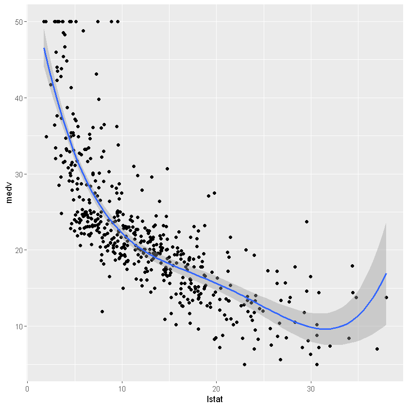
ggplot(Boston, aes(lstat, medv) ) +
  geom_point() +
  geom_smooth(method = lm, formula = y ~ poly(x, 4, raw = TRUE))
  

polynomial regression 4th power

Quantile regression

Quantile regression is an extension of linear regression used when the conditions of linear regression are not met. One advantage of quantile regression relative to ordinary least squares regression is that the quantile regression estimates are more robust against outliers in the response measurements.

Warning

For quantile regression to be feasible, dependent variable should have not many zeros or repeated values